2. Relational Algebra Without the Math
A plan is not a pile of operations. Its shape is part of the answer.
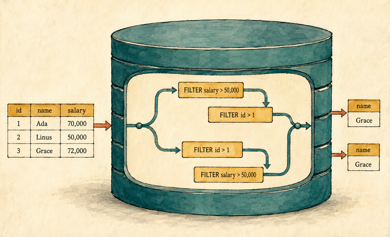
Chapter 1 left us with a working query engine and one unanswered question: how can we tell whether two query plans mean the same thing? This matters because databases often rearrange operations to perform less work. A different arrangement is useful only when it preserves the original answer. Before we can build an optimizer, we need a reliable way to distinguish safe transformations from incorrect ones.
To compare plans, we need a precise way to describe what each operation means. Relational algebra provides that language. We will introduce it through the employee rows and operations already present in our program, then use it to explain why one plan rearrangement preserves the result while another changes it.
Instead of adding another operator, this chapter uses the engine we already have. We will define equivalence, learn three laws for transforming the operators our engine supports, and use counterexamples to reject transformations that satisfy no valid law.
Build-along checkpoint
Begin with the completed Chapter 1 checkpoint:
git switch --create chapter-002 lesson-001This chapter does not require source changes. We will use the existing engine to compare plans and search for counterexamples. The
lesson-002tag is the completed Chapter 2 checkpoint.
2.1 We already have the pieces
Return to our first request: find the names of employees who earn more than 50,000. Ada and Grace appear in the result. Linus does not. Three operations produce that answer: a scan reads the rows, a filter applies a predicate, and a project keeps the requested columns.
Here is the request in ordinary language:
From the employees, keep those earning more than 50,000, then show only their names.
Each part corresponds to one plan node:
Project(name)
    ↑
Filter(salary > 50000)
    ↑
Scan(employees)
Read from the bottom upward. The scan supplies all three employee rows. The
filter’s predicate keeps Ada and Grace. The project removes id and salary
from those rows. Each node performs one small transformation, and its result
feeds the node above it.
The same structure could query products, books, or bank accounts. Only the source rows, predicate, and requested columns would change. This repeatable shape lets us compare plans instead of treating every query as unrelated code. Because a plan is an expression built from smaller expressions, we can ask whether changing its structure preserves its meaning.
2.2 Intermediate results are relations too
Chapter 1 introduced a relation as the table-shaped collection of rows on
which our engine operates. The original employees table is one relation:
| id | name | salary |
|---|---|---|
| 1 | Ada | 70,000 |
| 2 | Linus | 50,000 |
| 3 | Grace | 72,000 |
The important extension is that a relation does not need to be a stored table. After the filter runs, its two-row result is also a relation. After the project runs, its one-column result is another. An intermediate result may exist only long enough to feed the next operation, but it still has rows and columns.
This shared shape is what lets operations connect. A filter accepts a relation and produces a relation. A project does the same. The output of one operation can therefore become the input of another without changing into a completely different kind of value. That makes rearrangement possible, although it does not make every rearrangement correct.
Now we can name the two transformations more precisely.
2.3 Selection, projection, and logical plans
Our Filter keeps rows for which its predicate is true. Relational algebra
calls this operation selection and represents it with the Greek letter
σ, pronounced “sigma.” The predicate is written as a subscript, so
σsalary > 50000 means “keep rows whose salary is
greater than 50,000.”
The terminology can be confusing because SQL uses SELECT to choose output
columns. In relational algebra, selection chooses rows. Applied to our
employees, it produces:
| id | name | salary |
|---|---|---|
| 1 | Ada | 70,000 |
| 3 | Grace | 72,000 |
Our Project keeps named columns and removes the others. Relational algebra
calls this operation projection, represents it with π, pronounced “pi,”
and writes the retained columns as a subscript. Thus
πname means “keep the name column.”
| name |
|---|
| Ada |
| Grace |
Selection changes which rows continue. Projection changes which columns continue. Together with relations and rules for connecting operations, they form the small relational algebra that Chapter 1 uncovered. Our query can now be written as an algebra tree:
Projection: πname
             ↑
Selection:  σsalary > 50000
             ↑
Relation:   employees
The compact form contains the same nesting:
πname(σsalary > 50000(employees))
Read the inner operation first. Selection receives employees, and projection
receives the selection result. The symbols are useful shorthand, but the tree
often makes the flow easier to inspect.
This tree describes what result the query requires without choosing among algorithms for producing it. A description at this level is a logical plan. It lets us reason about the query independently of whether rows later come from memory, a file, or an index.
A physical plan describes how the database performs that logical work. For example, one logical scan might become a full table scan or an index scan. Our engine has no such alternatives yet, so a later Season 2 lesson will split logical and physical plans when there are real choices to represent.
For now, the Plan enum serves both roles. Its Scan is the leaf that brings
stored rows into execution, while its boxed inputs connect operations into the
same tree shown above. Chapter 1 already followed execute() through that
structure, so we do not need to draw it again. Once every node has a precise
meaning, two differently shaped trees can be compared by the relations they
produce.
Production note: Projection and duplicate rows
In textbook relational algebra, a relation is a set, so it cannot contain duplicate rows. Projection therefore removes duplicates. Our engine stores rows in a
Vec<Row>and produces one projected row for every input row. If two employees are named Ada,Project(name)returns two Ada rows. This is closer to SQL projection withoutDISTINCTthan to textbookπ.Chapter 1’s third experiment showed that reversing the input also reverses our output. That observation describes this
Vec<Row>implementation, not a promise made by the relational model, which does not define row order.
2.4 What makes two plans equivalent?
Suppose two different plan trees both return Ada and Grace for our current table. That is encouraging, but it does not prove that they mean the same thing. They may agree only because these three rows do not expose their difference. To rule out that possibility, we must compare them across every input that both plans can process.
A plan can run only when its input contains the columns and value types its operations require. We call an input valid for two plans when both plans can run on it. The plans are equivalent when they produce the same result for every such input. This prevents one convenient example from becoming a false proof.
For this chapter, the same result means the same number of rows in the same
order, with the same columns and values, including the same duplicates. Those
requirements describe what our current Vec<Row> engine exposes. Textbook
relations use set semantics and do not promise row order, so their definition
does not include all of these details.
The formal study of this question goes much deeper. Aho, Sagiv, and Ullman studied equivalence for expressions built from selection, projection, and join with query optimization in mind. Their method represents expressions with tableaux and can account for functional dependencies. This chapter uses only the small fragment justified by the operators and behavior our engine already has. See “Equivalences among Relational Expressions,” SIAM Journal on Computing, 1979.
2.5 Three equivalence laws we can use
An equivalence law describes a plan transformation that preserves the result whenever its conditions hold. The conditions matter as much as the shapes. A matching result for Ada, Linus, and Grace is evidence about one input; a law lets us reason about every valid input covered by its conditions.
These are not all the laws of relational algebra. They are the first three supported by selection, projection, and the deliberately narrow semantics of our engine.
2.5.1 Filters can exchange places
Consider two predicates, p and q:
Filter(p)              Filter(q)
   │                      │
Filter(q)      ≡       Filter(p)
   │                      │
   R                      R
A row reaches either root exactly when both predicates are true. The compact relational-algebra law is:
σp(σq(R)) ≡ σq(σp(R))
Both filters must be able to evaluate every input row. In our engine, that means each named column exists and contains an integer. Each filter then compares that integer with a fixed boundary without changing the row or anything else. Swapping the filters may change which predicate runs first, but it cannot change which rows satisfy both predicates.
2.5.2 Nested projections can collapse
Suppose projection A keeps a subset of the columns kept by projection B:
Project(A)              Project(A)
    │                       │
Project(B)      ≡           R
    │
    R
The inner projection removes nothing that the outer projection needs, so it cannot affect the final row:
πA(πB(R)) ≡ πA(R), when A ⊆ B
For our engine, A keeps the same final column order on both sides, and each
projection produces one output row for every input row. The law therefore also
preserves the duplicates and row order that our implementation exposes.
2.5.3 An early projection can remove unused columns
The final projection cannot simply move below the filter. The filter may need columns that do not belong in the final answer. Instead, we keep the final projection and introduce another projection below the filter:
Project(A)              Project(A)
    │                       │
Filter(p)       ≡       Filter(p)
    │                       │
    R               Project(A ∪ cols(p))
                            │
                            R
Let A be the columns required in the final result, and let cols(p) be the
columns read by predicate p. The lower projection must retain both groups:
πA(σp(R)) ≡ πA(σp(πA ∪ cols(p)(R)))
For the employee query:
A           = {name}
cols(p)     = {salary}
A ∪ cols(p) = {name, salary}
The lower projection may remove id, but it must preserve both name for the
answer and salary for the filter. Every column in A ∪ cols(p) must exist in
the input relation.
The lower projection removes only columns needed by neither the filter nor the final result. The filter therefore sees the same predicate values and makes the same decisions. The outer projection then returns the same final columns in the same order. This argument applies to every valid input, not only the table currently in front of us, and gives us a reusable criterion for the safe and unsafe rearrangements ahead.
2.6 Apply the laws
The order of nodes is part of a plan’s meaning. Moving an operation changes which columns and rows are available to the next operation. We can see the difference by trying one unsafe rearrangement and one safe one.
2.6.1 An unsafe projection
The working plan filters before removing columns. Now place
Project(name) below the filter:
Filter(salary > 50000)
       │
Project(name)
       │
Scan(employees)
We already know that data moves from the bottom toward the root, so plain lines
can now stand for that flow. The scan supplies complete rows, but the project
removes salary. When the filter receives those smaller rows, its predicate
asks for a column that no longer exists. Our engine stops with
unknown column: salary.
The nodes have familiar names, but the plan cannot perform the request. This
transformation does not satisfy the projection law because the lower project
omits salary, a column in cols(p). A rearrangement is valid only if every
operation still receives the information it needs.
2.6.2 A safe projection
Removing columns early was not the mistake. Removing a required column was.
An early projection may discard id while retaining name for the final
answer and salary for the predicate:
Original                         Remove id early

Project(name)                    Project(name)
       │                                │
Filter(salary > 50000)           Filter(salary > 50000)
       │                                │
Scan(employees)                  Project(name, salary)
                                        │
                                 Scan(employees)
Here, A is {name} and cols(p) is {salary}. Their union is
{name, salary}, exactly what the lower project retains. The filter can still
read salary, and the upper project still returns name. The transformation
satisfies the projection law, so its correctness does not depend on Ada,
Linus, or Grace.
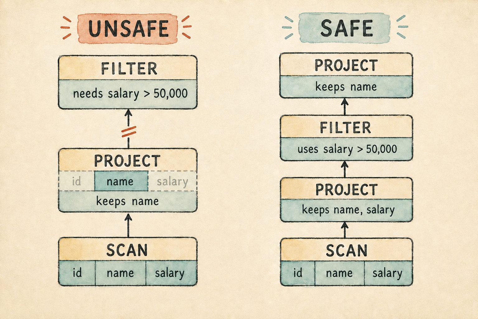
We have justified one meaning-preserving transformation. We have not taught the database to discover or apply it. Automatic rewriting belongs to the optimizer we will build in Season 3.
2.6.3 A counterexample
Testing several inputs can expose an invalid claim. Suppose one plan contains two salary filters while another accidentally drops the stricter filter:
Both filters                     Stricter filter dropped

Filter(salary > 60000)           Filter(salary > 50000)
          │                                │
Filter(salary > 50000)           Scan(employees)
          │
Scan(employees)
Both plans return Ada and Grace for our original table. Neither table contains a salary between 50,000 and 60,000, so the missing condition appears harmless. Now add Edsger:
| id | name | salary |
|---|---|---|
| 4 | Edsger | 55,000 |
The first plan removes Edsger; the second keeps him. This row is a counterexample, one valid input that proves the plans are not equivalent. Equivalence requires agreement for every valid input, so one disagreement is enough to reject the transformation. An optimizer may not use it as a general rewrite rule.
There is a redundant condition in the first plan, but it is the weaker one. Any salary greater than 60,000 is already greater than 50,000. We learn which condition is removable from their meanings, not from the particular rows in our first table.
Passing examples are not a general proof. A law and its conditions justify a transformation; a counterexample rejects a false one.
2.7 Why equivalent plans matter
A database often has several ways to answer the same query. One plan may remove unused columns early. Another may delay that work. Joins will eventually create choices with much larger consequences. Different arrangements may process fewer rows, use less memory, or finish sooner.
An optimizer does not rearrange plans arbitrarily. It applies transformations whose equivalence conditions are known to hold. A fast plan that returns different rows is not an optimization. It is a bug. Equivalence is the safety boundary: change the shape as much as useful, but do not change the meaning.
Season 3 will turn that freedom into a query optimizer. It will apply rewrite rules, estimate costs, and choose among equivalent alternatives. Correctness comes first because the optimizer can choose only among plans that preserve the query’s meaning.
2.8 What we deliberately did not build
This chapter gives our small plans a logical interpretation, but the engine is still intentionally incomplete:
- It does not separate logical nodes from physical execution algorithms.
- It cannot discover or apply equivalent-plan rewrites automatically.
- It has no statistics or cost model for choosing a faster plan.
- Its
Vec<Row>preserves row order and permits duplicate rows, unlike a mathematical relation. - Its
Projectpreserves duplicates instead of implementing textbookπ. - Its predicates only read a column and compare an integer. We have not introduced nulls, expressions that can fail while being evaluated, functions that may return a different answer each time, or expressions that change data or other state.
- We did not implement the paper’s tableaux or its procedures for deciding equivalence.
- We have not introduced joins or functional dependencies, even though both belong to the broader formal treatment.
- These three laws do not cover full relational algebra or SQL. Additional operators and different duplicate semantics can add conditions to otherwise familiar transformations.
Those missing predicate behaviors matter to equivalence. An expression might fail because it divides by zero or converts invalid text. A function based on the current time or a random value may not return the same answer twice. An expression that changes data, increments a counter, or writes output changes something beyond its own true-or-false result. If predicates can behave in these ways, swapping two filters may change which failures or changes occur. The filter law therefore needs more conditions in a richer language than it does in our current engine.
These limitations matter, but solving them together would hide the idea we needed first. This chapter asks whether a transformation is correct. Later lessons can ask how to represent alternatives, find them, and choose among them.
2.9 Try it
Use the current Plan, Row, and Value types as a concrete model for these
experiments. Try to decide each answer before opening the explanation.
- Build two filters,
salary > 50000andid > 1, then swap their order. Which law permits the transformation, and which conditions does it assume? - Place a projection below those two filters. Use the projection law to find the smallest set of columns it must retain while still returning names.
- Explain which condition is violated when
Project(name)is placed belowFilter(salary > 50000). - Remove one filter from the two-filter plan in Section 2.6.3. Find the smallest counterexample that shows the new plan is not equivalent.
- Add two employees named Ada and run
Project(name). How does the result differ from textbookπ?
Check your reasoning
- Filters can exchange places. Both predicates must be deterministic, valid for the input rows, free of side effects, and able to read their columns.
- The final result needs
name, while the predicates needsalaryandid. Their union is{name, salary, id}, so nothing can be removed from our three-column rows. - The projection law requires the lower project to retain
cols(p). Keeping onlynameremovessalary, so the filter cannot evaluate its predicate. - One employee earning 55,000 is enough. The two-filter plan removes that
row, while the plan containing only
salary > 50000keeps it. - Our project returns two identical
{name: "Ada"}rows. Textbook projection produces one because mathematical relations do not contain duplicates.
2.10 From SQL to a plan
We can now assign meaning to a small logical plan, apply three justified
transformations, and reject a false one with a counterexample. Yet every plan
in the program is still assembled from Rust enum values. A person should not
need to write Box::new(Plan::Filter { ... }) merely to ask for employee
names.
SQL provides a convenient way to express the request. Its words and punctuation are not the plan itself. They are source text from which the database can build a plan. The plan carries the meaning we studied here, regardless of the text that produced it.
That separation creates our next problem. How does a database turn characters
such as SELECT, FROM, and WHERE into the tree our engine knows how to
execute? The next lesson builds the smallest SQL frontend needed to answer
that question.